Example Applications

In the following, we will explore how GinJinn2 can be applied to automatically detect structures in several empirical contexts.

Seed Counting

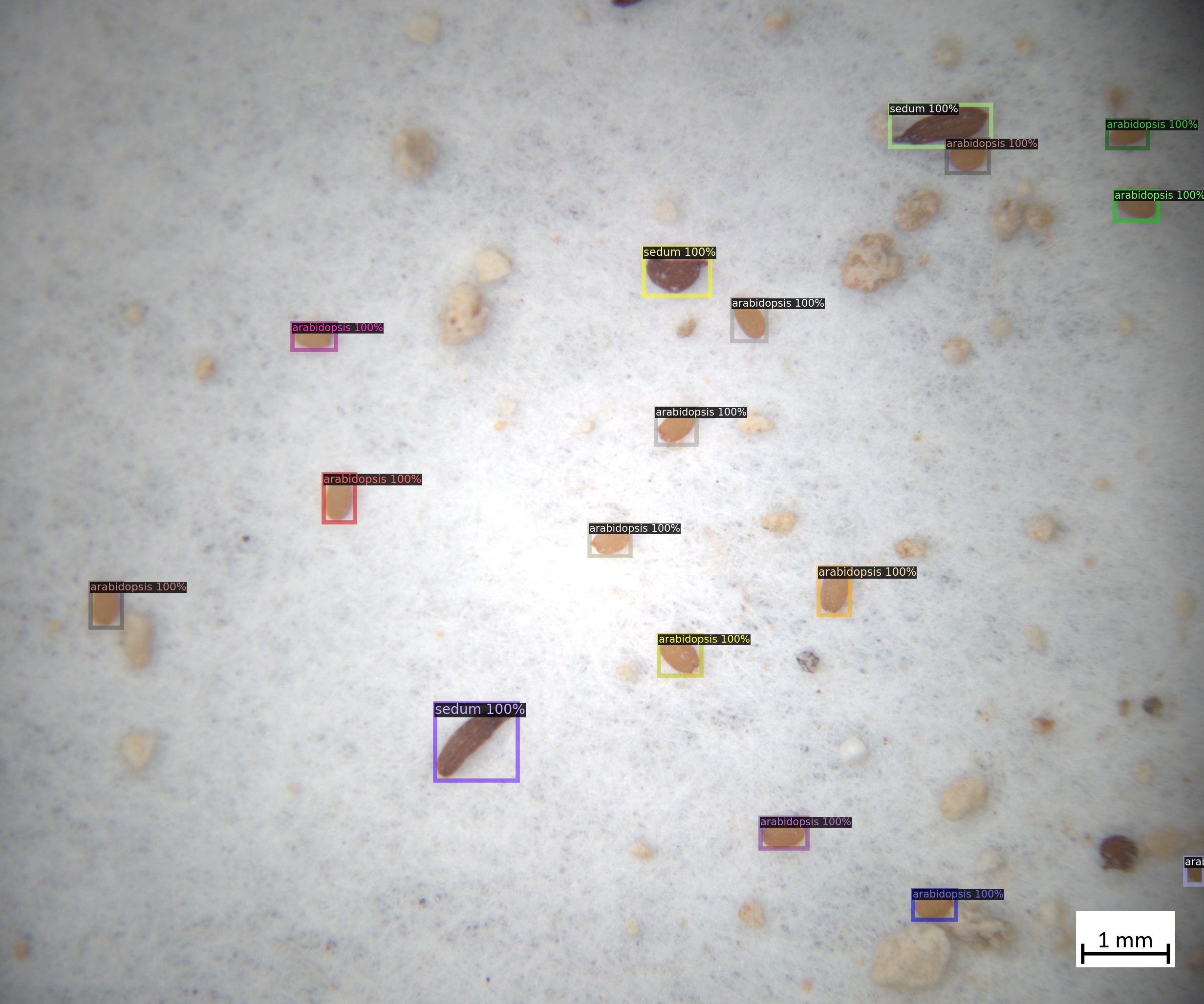
The seeds dataset comprises microscopic images of sand-contaminated seed mixtures of the plant genera Sedum and Arabidopsis. The seeds are annotated with bounding-boxes and labeled according to their genus membership. Such a dataset might be analyzed for quality control purposes, i.e., to assess if the composition of a commercial seed mixture is as expected. Another possible scenario is the analysis of ecological samples such as seeds collected with seed traps. In the following, we will train a model to automatically detect seeds and determine their genus, and finally quantify the composition of seed mixtures.

An example image overlaid with object annotations:

Seed image with bounding-box annotations.

Data preparation

First the dataset must be downloaded and prepared to be used as an input for GinJinn2.

Download the data:

The dataset in COCO format is available from GFBio at https://doi.org/10.34656/k53b-9c27.1.

Download and unzip from the commandline:
```
wget https://data.bgbm.org/dataset/gfbio/0035/gfbio0035.zip
mkdir seeds_raw
unzip gfbio0035.zip -d seeds_raw
```
The extracted files are now located in the “seeds_raw” directory. This is already a GinJinn2-compatible COCO dataset comprising an images directory being sibling to an annotations.json file.
Train-Validation-Test split:

It is a good practice in Machine Learning (ML) to split the available labeled data into sub-datasets for training, validation, and testing. This enables to assess the performance of a trained ML model on unseen data. The general idea is to use the training dataset for model training, the validation (sometimes called “development”) dataset for hyper-parameter tuning, and, finally, the test dataset as a proxy for the real-world performance of the model. For this purpose, GinJinn2 provides the ginjinn split command. This command uses a heuristic to generate sub-datasets whose object occurrences aim to be representative for the original dataset.

Split the dataset into sub-datasets for training (60%), test (20%), and validation (20%):
```
ginjinn split -I seeds_raw -o seeds_split -d bbox-detection -t 0.2 -v 0.2
```

Now the dataset is ready to be used for model training.

Model fitting

Generate new GinJinn2 project:

First, we need to generate a new GinJinn2 project using the ginjinn new command. You can provide a model template (-t), and a data directory (-d) to this command. Here, we will use a Faster R-CNN as detection model, and the previously generated split dataset as data directory.
```
ginjinn new seeds_project -t faster_rcnn_R_101_FPN_3x.yaml -d seeds_split
```
This will create the folder seeds_project, containing a ginjinn_config.yaml file and an outputs folder.

Modify project configuration:

Now, we will modify the number of training iterations, the evaluation period, and the checkpointing period. Additionally, we will add several optional data augmentations. These are randomized data transformations (e.g. varying rotation, contrast, etc.) that are applied to the images and annotations prior to their use for model training. In this way, the dataset is artificially enlarged and made more variable, which very often leads to better model performance on new data.

In ginjinn_config.yaml we will set the entries:

# ...
training:
    # ...
    max_iter: 7000
    eval_period: 250
    checkpoint_period: 1000
# ...
augmentation:
   - horizontal_flip:
       probability: 0.25
   - vertical_flip:
       probability: 0.25
   - brightness:
       brightness_min: 0.8
       brightness_max: 1.2
       probability: 0.25
   - contrast:
       contrast_min: 0.8
       contrast_max: 1.2
       probability: 0.25
   - saturation:
       saturation_min: 0.8
       saturation_max: 1.2
       probability: 0.25
   - rotation_range:
       angle_min: -30
       angle_max: 30
       expand: True
       probability: 0.25

The project is now ready for training.

Train and validate model:

Model training is started via
```
ginjinn train seeds_project
```
While this command is running, several files will be generated in the seeds_project/outputs directory. The periodically updated file seeds_project/outputs/metrics.pdf will contain various metrics (e.g. losses, AP) referring to the training or validation dataset and can be used to monitor the training progress.
Evaluate trained model:

After training, the model can be evaluated using the test dataset by executing the command
```
ginjinn evaluate seeds_project
```
This will write the evaluation output to seeds_project/evaluation.csv. If there is a large discrepancy between the final validation metrics (see seeds_project/outputs/metrics.pdf or metrics.json) and the evaluation output, there is most likely a problem with the model.

Prediction and counting

Now, we can use the trained model to predict bounding-boxes enclosing seeds and their respective genus for new image data. As stand-in for new data, we will use the previously generated test dataset as input to the ginjinn predict command. We will also turn on the visualization option (-v) to get a visual representation of the predictions.

ginjinn predict seeds_project -i seeds_split/test/images -o seeds_test_prediction -v

This will generate a COCO dataset named seeds_test_prediction. This dataset can be used as an input for all other GinJinn2 commands supporting COCO input. The visualizations are written to seeds_test_prediction/visualization.

The visualization of the predictions will look similar to this:

Seed image with predicted bounding boxes.

Finally, we will use the ginjinn utils count command to count the number of seeds per genus for each image:

ginjinn utils count -a seeds_test_prediction/annotations.json -o seeds_test_prediction/counts.csv

This will write the image-wise seed counts to seeds_test_prediction/counts.csv. Based on this file, the proportion of seeds from both genera can be calculated using any tool with CSV-reading capability (e.g. EXCEL, R, Python, …).

Insect Monitoring using Glue Traps

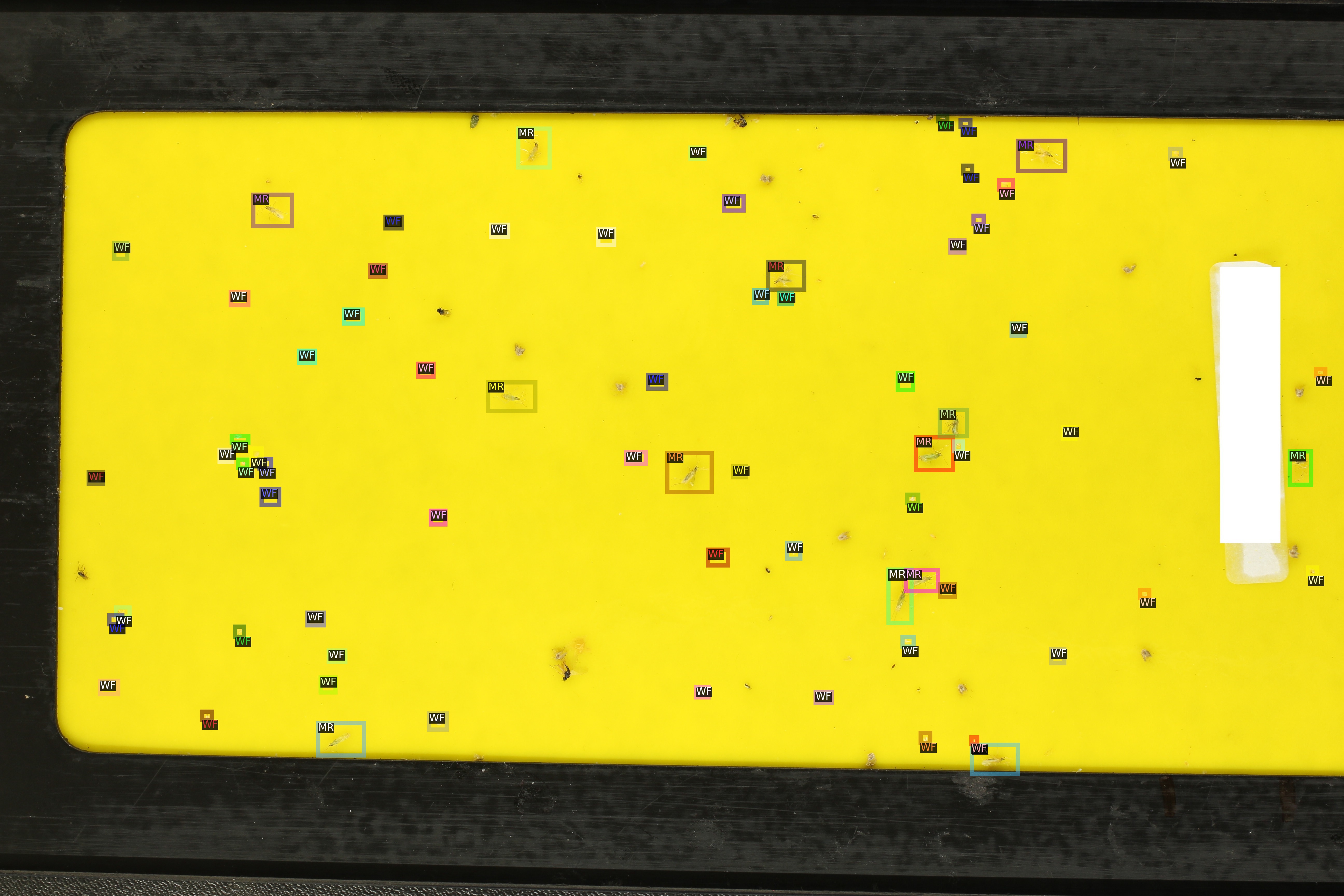
The Yellow-Stickytraps dataset comprises images of yellow glue traps placed in greenhouses. Three categories of insects are annotated with bounding boxes: Whiteflies (WF), Nesidiocoris (NC), and Macrolophus (MC). Our goal is to automate the counting of insects per category. This may, for example, be useful for evaluating the effectiveness of pest control measures.

The Yellow-Stickytraps dataset has some potentially problematic properties:

Objects (insects) are very small compared to the image size.
Bounding box annotations are relatively loose.
The contrast between background and insects is relatively low.

We will mitigate problem 1) by splitting the original images into sliding windows, which will be used as input for a bounding-box object detection model. Problems 2) and 3) could be addressed by a more careful annotation scheme and image preprocessing, respectively. Those, however, will not be discussed in this section.

In the following, we will train a model to automatically detect, categorize, and count insects.

An example image overlaid with object annotations:

Yellow-Stickytraps image with bounding-box annotations.

General data preparation

First the dataset must be downloaded and prepared to be used as an input for GinJinn2.

Download the data:

The dataset in COCO format is available from GFBio at https://doi.org/10.34656/41pk-rn18.1.

Download and unzip from the commandline:
```
wget https://data.bgbm.org/dataset/gfbio/0036/gfbio0036.zip
mkdir stickytraps_raw
unzip gfbio0036.zip -d stickytraps_raw
```
The extracted files are now located in the “stickytraps_raw” directory.

Flatten the COCO dataset:

This makes sure all images are located in the same directory:

ginjinn utils flatten -i stickytraps_raw/images -a stickytraps_raw/annotations.json -o stickytraps_flat

Train-Validation-Test split:

We split the Yellow-Stickytraps dataset into sub-datasets for training (60%), test (20%), and validation (20%). For this dataset, it may be necessary to generate multiple split proposals until the category proportions are sufficiently homogeneous across the sub-datasets.
```
ginjinn split -I stickytraps_flat -o stickytraps_split -d bbox-detection -t 0.2 -v 0.2
```

Sliding-window cropping

We will now apply Sliding-Window Cropping to be able to detect the small insects fixed on relatively large glue traps. The following command will split the original images into sliding windows of 1024x1024 pixels in size (-s 1024) with an overlap of 256 pixels (-p 256) between neighboring sliding windows. Annotations that are incomplete after the splitting, i.e. “cut-off” polygons, will be excluded (-c). The sliding-window split should be done in the context of bounding box detection (-k bbox-detection).

ginjinn utils sw_split -I stickytraps_split -o stickytraps_split_sw -s 1024 -p 256 -k bbox-detection -c

Model fitting

Generate new GinJinn2 project:

First, we need to generate a new GinJinn2 project using the ginjinn new command. You can provide a model template (-t) and a data directory (-d) to this command. Here, we will use a Faster R-CNN as object detection model, and the previously generated split dataset as data directory.
```
ginjinn new stickytraps_project -t faster_rcnn_R_101_FPN_3x.yaml -d stickytraps_split_sw
```
This will create the folder stickytraps_project, containing a ginjinn_config.yaml file and an outputs folder.

Modify project configuration:

Now, we will modify the number of training iterations, the evaluation period, and the checkpointing period. Additionally, we will add several optional data augmentations. These are randomized data transformations (e.g. varying rotation, contrast, etc.) that are applied to the images and annotations prior to their use for model training. In this way, the dataset is artificially enlarged and made more variable, which very often leads to better model performance on new data.

In ginjinn_config.yaml we will set the entries:

# ...
training:
    # ...
    max_iter: 7000
    eval_period: 250
    checkpoint_period: 1000
# ...
augmentation:
   - horizontal_flip:
       probability: 0.25
   - vertical_flip:
       probability: 0.25
   - brightness:
       brightness_min: 0.8
       brightness_max: 1.2
       probability: 0.25
   - contrast:
       contrast_min: 0.8
       contrast_max: 1.2
       probability: 0.25
   - saturation:
       saturation_min: 0.8
       saturation_max: 1.2
       probability: 0.25
   - rotation_range:
       angle_min: -30
       angle_max: 30
       expand: True
       probability: 0.25

The project is now ready for training.

Train and validate model:

Model training is started via
```
ginjinn train stickytraps_project
```
While this command is running, several files will be generated in the stickytraps_project/outputs directory. The periodically updated file stickytraps_project/outputs/metrics.pdf will contain various metrics (e.g. losses, AP) referring to the training or validation dataset and can be used to monitor the training progress.
Evaluate trained model:

After training, the model can be evaluated using the test dataset by executing the ginjinn evaluate command:
```
ginjinn evaluate stickytraps_project
```
This will write the evaluation output to stickytraps_project/evaluation.csv. If there is a large discrepancy between the final validation metrics (see stickytraps_project/outputs/metrics.pdf or metrics.json) and the evluation output, there is most likely a problem with the model.

Prediction and counting

Now, we can use the trained model to predict bounding boxes and insect categories on new image data. As stand-in for new data, we will use the previously generated test dataset as input to the ginjinn predict command. We will also turn on the visualization option (-v), to get a visual representation of the predictions.

ginjinn predict stickytraps_project -i stickytraps_split_sw/test/images -o stickytraps_test_prediction -v

This will generate a COCO dataset named stickytraps_test_prediction, which can be used as an input for all other GinJinn2 commands supporting COCO input. The visualizations are written to stickytraps_test_prediction/visualization.

Before we can count the insects, we first need to remove duplicated objects. Duplications occur when an object is present in two or more sliding windows and successfully detected in more than one of them. We will use ginjinn utils sw_merge to combine the predictions for sliding windows as this will automatically remove duplicate predictions. The following command merges the sliding-window images (-i stickytraps_split/test/images) and annotations (-a stickytraps_test_prediction/annotations.json), and writes the merged images and annotations to stickytraps_test_prediction_merged (-o).

ginjinn utils sw_merge -i stickytraps_split_sw/test/images -a stickytraps_test_prediction/annotations.json -o stickytraps_test_prediction_merged -t bbox-detection

If you want to have a look at the predictions, the results can be visualized using ginjinn vis -I stickytraps_test_prediction_merged -v bbox.

The visualization of the predictions based on the sliding windows will look similar to this:

Sliding-window image of the Yellow-Stickytraps dataset with predicted bounding boxes.

Now that duplicate predictions are removed, we can count the insects:

ginjinn utils count -a stickytraps_test_prediction_merged/annotations.json -o stickytraps_test_prediction_merged/counts.csv

This will write the image-wise insects counts to stickytraps_test_prediction_merged/counts.csv, which can be processed using any tool with CSV-reading capability (e.g. EXCEL, R, Python, …).

Leucanthemum Leaf Segmentation

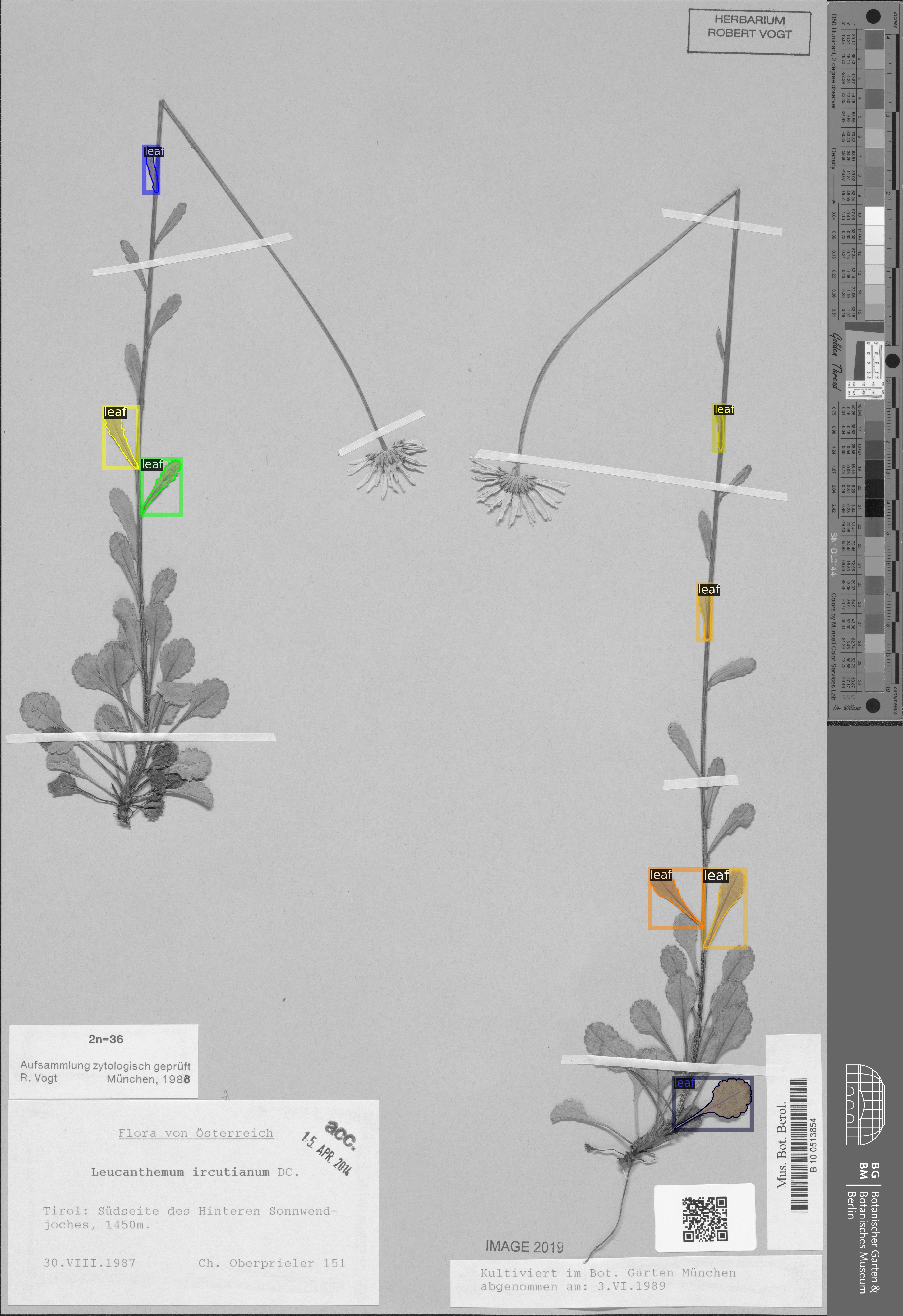
The Leucanthemum dataset comprises images of herbarium specimens from 12 Leucanthemum species. There is only one object category “leaf”, which denotes intact leaves that could be used to quantify leaf shape, e.g., for geometric morphometrics. To be able to train a segmentation model for pixel-perfect detection, the leaves are annotated using polygons.

An example image with overlaid object annotations (here, the image is shown in grayscale to emphasize the annotations):

Leucanthemum image with instance-segmentation annotations.

Using this dataset, we will build a pipeline to facilitate automatic feature extraction from digitized herbarium specimens. Similar to the Yellow-Stickytraps dataset, there are some potential problems concerning the data:

The objects (leaves) are small in relation to the image size.
The images are very large (~4000x6000 pixels).
The objects (leaves) are very variable (basal vs. apical leaves).

Problem 3) could potentially be solved by subdiving the leaf category into subcategories like apical, intermediate, and basal leaves. This, however, would potentially require a larger amount of training data to account for the now smaller number of samples per category. We will concentrate on solving problems 1) and 2) by applying a custom pipeline consisting of two models: The first model, from now on called BBox Model, will be trained to detect the bounding boxes of intact leaves in sliding-window crops of the original images. The second model, from now on called Segmentation Model (Seg. Model), will segment the leaves within the bounding boxes.

The pipeline for model fitting will look like this:

Leucanthemum leaf segmentation pipeline.

Data preparation

First the dataset must be downloaded and prepared to be used as an input for GinJinn2.

Download the data:

The dataset in COCO format is available from GFBio at https://doi.org/10.34656/skvz-cs62.1.

Download and unzip from the commandline:
```
wget https://data.bgbm.org/dataset/gfbio/0034/gfbio0034.zip
mkdir leucanthemum_raw
unzip gfbio0034.zip -d leucanthemum_raw
```
The extracted files are now located in the “leucanthemum_raw” directory.
Flatten the COCO dataset:

GinJinn2 expects all images to be placed directly in the folder images within the dataset folder an as a sibling of the annotations (annotations.json for COCO or annotations folder for Pascal-VOC). To transform any valid COCO dataset into a flat COCO dataset, GinJinn2 provides the ginjinn utils flatten command.

To flatten the Leucanthemum dataset:
```
ginjinn utils flatten -i leucanthemum_raw/images -a leucanthemum_raw/annotations.json -o leucanthemum_flat
```

Further cleaning:

Before proceeding with the analysis, let’s have a look into the flattened dataset with ginjinn info -I leucanthemum_flat:

# images: 303

category distribution:
           #seg  #bbox  total
leaf        915      0    915
main_vein     0      0      0
total       915      0    915

WARNING: Found categories without annotation
        - "main_vein"

The annotation file specifies two object categories “leaf” and “main_vein” comprising 915 and 0 objects, respectively. Since we are only interested in leaves and there are no annotations for “main_vein”, we will discard the latter object category:

ginjinn utils filter_cat -o leucanthemum_filtered -a leucanthemum_flat/annotations.json -i leucanthemum_flat/images -f leaf

ginjinn info -I leucanthemum_filtered now yields

# images: 295

category distribution:
       #seg  #bbox  total
leaf    915      0    915
total   915      0    915

Train-Validation-Test split:

It is a good practice in Machine Learning (ML) to split the dataset into sub-datasets for training, validation, and testing. This is necessary to be able to assess the performance of a trained ML on unseen data. The general idea is to use the training dataset for model training, and the validation (sometimes called “development”) dataset for hyper-parameter tuning, and finally the test dataset as a proxy for real-world performance of the model. For this purpose, GinJinn2 provides the ginjinn split command. This command uses a heuristic to generate sub-datasets whose object occurrences aim to be representative for the original dataset.

Split the Leucanthemum dataset into train (60%), test (20%), and validation (20%):
```
ginjinn split -I leucanthemum_filtered -o leucanthemum_split -d instance-segmentation -t 0.2 -v 0.2
```

Bounding Box Model

Sliding-window splitting

Similar to the Yellow-Stickytraps analysis, we will split the dataset into sliding windows. This time, however, we will use larger windows (-s 2048) with a larger overlap (-p 512):

ginjinn utils sw_split -I leucanthemum_split -o leucanthemum_split_sw -s 2048 -p 512 -c

The sliding windows will be used to train the detection model. Since the latter should only learn to detect complete, intact leaves, we use the -c/--remove_incomplete option to discard annotations of trimmed leaves.

Model training

Generate new GinJinn2 project:

ginjinn new leucanthemum_bbox -t faster_rcnn_R_101_FPN_3x.yaml -d leucanthemum_split_sw

Modify project configuration:

In leucanthemum_bbox/ginjinn_config.yaml we will set the entries:

# ...
training:
    # ...
    max_iter: 5000
    eval_period: 250
    checkpoint_period: 2500
# ...
augmentation:
   - horizontal_flip:
       probability: 0.25
   - vertical_flip:
       probability: 0.25
   - brightness:
       brightness_min: 0.8
       brightness_max: 1.2
       probability: 0.25
   - contrast:
       contrast_min: 0.8
       contrast_max: 1.2
       probability: 0.25
   - saturation:
       saturation_min: 0.8
       saturation_max: 1.2
       probability: 0.25
   - rotation_range:
       angle_min: -30
       angle_max: 30
       expand: True
       probability: 0.25

Train and validate model

Model training is started via:
```
ginjinn train leucanthemum_bbox
```
During the training process, several files will be generated in the leucanthemum_bbox/outputs directory. The periodically updated file leucanthemum_bbox/outputs/metrics.pdf will contain various metrics (e.g. losses, AP) referring to the training or validation dataset and can be used to monitor the training progress.
Evaluate trained model
```
ginjinn evaluate leucanthemum_bbox
```
This will write the evaluation output to leucanthemum_bbox/evaluation.csv. If there is a large discrepancy between the final validation metrics (see leucanthemum_bbox/outputs/metrics.pdf or metrics.json) and the evaluation output, there is most likely a problem with the model.
(Optional) Prediction, merging, visualization.

See ginjinn predict, ginjinn utils sw_merge, ginjinn visualize documentation, or Yellow-Stickytraps.

Segmentation Model

Bounding box cropping

To train a model to segment leaves within their already known bounding boxes, we first need to process the Leucanthemum dataset. Ginjinn provides the ginjinn utils crop command, which crops bounding boxes or polygons from annotated images, and generates a new annotation referring to the cropped images. The cropped images can then be used for model training. Here, we will crop the leaf bounding boxes with an additional margin (padding) of 25 pixels (-p 25) to account for some variation surrounding the leaves.

ginjinn utils crop -I leucanthemum_split -o leucanthemum_split_cropped -p 25 -t segmentation

Model training

Generate new GinJinn2 project:

ginjinn new leucanthemum_seg -t mask_rcnn_R_101_FPN_3x.yaml -d leucanthemum_split_cropped

Modify project configuration:

In leucanthemum_seg/ginjinn_config.yaml we will set the entries:

# ...
training:
    # ...
    max_iter: 5000
    eval_period: 250
    checkpoint_period: 2500
# ...
augmentation:
   - horizontal_flip:
       probability: 0.25
   - vertical_flip:
       probability: 0.25
   - brightness:
       brightness_min: 0.8
       brightness_max: 1.2
       probability: 0.25
   - contrast:
       contrast_min: 0.8
       contrast_max: 1.2
       probability: 0.25
   - saturation:
       saturation_min: 0.8
       saturation_max: 1.2
       probability: 0.25
   - rotation_range:
       angle_min: -30
       angle_max: 30
       expand: True
       probability: 0.25

Train and validate model

Model training is started via:
```
ginjinn train leucanthemum_seg
```
While this command is running, several files will be generated in the leucanthemum_seg/outputs directory. The periodically updated file leucanthemum_seg/outputs/metrics.pdf will contain various metrics (e.g. losses, AP) referring to the training or validation dataset and can be used to monitor the training progress.
Evaluate trained model
```
ginjinn evaluate leucanthemum_seg
```
This will write the evaluation output to leucanthemum_seg/evaluation.csv. If there is a large discrepancy between the final validation metrics (see leucanthemum_seg/outputs/metrics.pdf or metrics.json) and the evaluation output, there is most likely a problem with the model.
(Optional) Predict and visualize

We might be interested in how the model predictions look like:
```
ginjinn predict leucanthemum_seg -i leucanthemum_split_cropped/test/images -o leucanthemum_seg_test_prediction -v -c
```
The predictions will probably not look very convincing right now. To improve the segmentations, we can make use of the segmentation refinement option (-r) of the ginjinn predict command. This will use CascadePSP for improving the segmentations. This refinement is typically beneficial when object borders are relatively pronounced.
```
ginjinn predict leucanthemum_seg -i leucanthemum_split_cropped/test/images -o leucanthemum_seg_test_prediction_refined -v -c -r
```
The new predictions should look much better.

Visualizations of the predictions might look like this:

Making predictions

With both models trained, we can now run the leaf extraction pipeline. To predict on new data, the following steps are required:

Split new images into sliding windows
Predict from BBox Model to get leaf bounding boxes
Predict from Seg. Model on bounding boxes

For demonstration purposes, we will pretend that the test images are newly collected images.

cp -r leucanthemum_split/test/images new_images

First, the new images need to be split into sliding windows. Size (-s 2048) and overlap (-p 512) should be same as for the training data.

ginjinn utils sw_split -i new_images -o new_data_sw -s 2048 -p 512

Now, we predict the bounding boxes of the leaves using the BBox Model.

ginjinn predict leucanthemum_bbox -i new_data_sw -o new_data_sw_pred -v

To remove (merge) duplicated predictions within the overlap of neighboring windows, we can use sw_merge, which kind of reverts the sliding-window split.

ginjinn utils sw_merge -a new_data_sw_pred/annotations.json -i new_data_sw -o new_data_sw_pred_merged -t bbox-detection

These (merged) leaf bounding boxes are now cropped from the (reconstructed) original images. We also add some padding (-p 25), since we did the same when cropping the training images for the Seg. Model.

ginjinn utils crop -I new_data_sw_pred_merged -o new_data_sw_pred_merged_cropped -t bbox -p 25

Finally, we can use the cropped bounding boxes as input for the Seg. Model.

ginjinn predict leucanthemum_seg -i new_data_sw_pred_merged_cropped/images -o new_data_seg_pred -v -c -r

The predicted leaf masks (new_data_seg_pred/masks_cropped) can, for example, be used to quantify the leaf shape using geometric morphometrics.

The masks should look like this:

Visualization of the Leucanthemum workflow prediction.